Supplementary material
This page contains supplementary material for some tutorials and papers.
Tutorials on Visualization in multiobjective optimization
GECCO 2020
- Download tutorial slides and approximation sets.
GECCO 2019
- Download tutorial slides and approximation sets.
GECCO 2018
- Download tutorial slides and approximation sets.
CEC 2017
- Download tutorial slides.
GECCO 2016
- Download tutorial slides.
DEMO
DEMO (Differential Evolution for Multiobjective Optimization) is an algorithm based on Differential Evolution for solving multiobjective optimization problems. You can download its source code here (v1.3).
First experiments (EMO 2005)
In the first set of experiments, DEMO was compared to some other algorithms on five ZDT test problems. Here you can find the respective results:
- ZDT1 Pareto front and Pareto front approximation found by DEMO
- ZDT2 Pareto front and Pareto front approximation found by DEMO
- ZDT3 Pareto front and Pareto front approximation found by DEMO
- ZDT4 Pareto front and Pareto front approximation found by DEMO
- ZDT5 Pareto front and Pareto front approximation found by DEMO
Archive contents
Each archive file called `ZDTn_DEMO.zip` contains the approximation sets in the form `ZDTn.DEMO.X.Y.Z.set`, where:

- n is the ZDT problem number

- X means the applied DEMO variant:
    parent      = DEMO/parent
    closest_dec = DEMO/closest/dec
    closest_obj = DEMO/closest/obj

- Y stands for the used crossover probability:
    c30 = crossover probability 30%
    c60 = crossover probability 60%
    c90 = crossover probability 90%

- Z denotes the run (from 01 to 10)

The population size was 100 and the number of generations was 250 in all the experiments.

The file `ZDTn.DEMO.metrics` contains the generational distance, convergence and diversity metric values for each approximation set.
Further experiments (EMO 2007)
A second set of experiments on DTLZ and WFG test problems was performed to enable a better comparison between DEMO and state-of-the-art algorithms for multiobjective optimization (NSGA-II, SPEA2 and IBEA). We experimented with DEMO in four variants that differ only in the chosen environmental selection:
- DEMO NS-II uses environmental selection from NSGA-II
- DEMO SP2 uses environmental selection from SPEA2
- DEMO IB eps uses environmental selection from IBEA with the eps indicator
- DEMO IB hd uses environmental selection from IBEA with the hd indicator
DEMO with the chosen environmental selection was compared to the respective genetic algorithm on 7 DTLZ problems and 9 WFG problems (each using 2, 3 and 4 objectives) with the following outcomes:
Archive contents
Each archive file called `ALG.zip` contains the approximation sets of ALG and DEMO's variant corresponding to ALG for the problems DTLZ and WFG.

The files in the archive containing the approximation sets have the form `X.Y.Z`, where:

- X stands for the problem:
    DTLZ1
    DTLZ2
    DTLZ3
    DTLZ4
    DTLZ5
    DTLZ6
    DTLZ7
    WFG1
    WFG2
    WFG3
    WFG4
    WFG5
    WFG6
    WFG7
    WFG8
    WFG9

- Y stands for the algorithm:
    demo_alg
    alg

- Z denotes the the number of objectives:
    m2 = 2 objectives
    m3 = 3 objectives
    m4 = 4 objectives

In all experiments, the population size was set to 100 and 300 generations were evolved. Each algorithm was run 30 times on each problem.
BBDEMO
The BBDEMO (Black-Box Differential Evolution for Multiobjective Optimization) algorithm was inspired by the BBDE and COMO-CMA-ES algorithms and was made for solving mixed-integer problems.
You can download the source code of the BBDEMO algorithm as well as the results achieved by BBDEMO and Random Search on the bbob-mixint-biobj test problems of the COCO platform (COCO archive definition).
Visualization with prosections
With prosections (projections of a section), 4-D approximation sets can be plotted in 3-D in a simple and intuitive way.
First examples (GECCO 2011)
Visualizing 4-D approximation sets using prosections works like this:
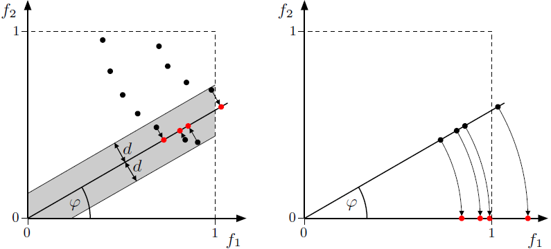
Choose the 2-D projection plane (for the sake of simplicity, let us assume this is \(f_1f_2\)), angle \(\phi\) and distance \(d\). These parameters define the section (the gray area in the left figure below).
All vectors within this section are first orthogonally projected to the line crossing the origin and intersecting the \(f_1\)-axis at angle \(\phi\), and finally rotated. For these transformations, one of the following functions is used:
3-D case:
\[(f_1, f_2, f_3) \mapsto (f_1 \cos\phi + f_2 \sin\phi, f_3)\]
4-D case:
\[(f_1, f_2, f_3, f_4) \mapsto (f_1 \cos\phi + f_2 \sin\phi, f_3, f_4)\]
The prosections are denoted as 3D(\(f_1f_2, \phi, d\)) and 4D(\(f_1f_2, \phi, d\)), respectively.
All vectors outside the section are ignored.
Visualizing a discontinuous front
For this example, we use an approximation set of discontinuous shape (as in the DTLZ7 test problem).
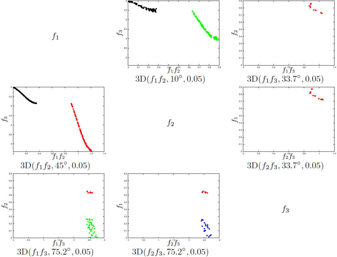
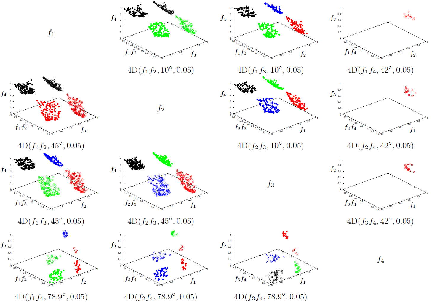
Using gnuplot we can make an animation of the prosection matrix with angles going from 0° to 90°:
- 3-D case: data files and gnuplot scripts
- 4-D case: data files and gnuplot scripts
Archive contents
The archive `nd.data.zip` (where n is either 3 or 4) contains:

- Approximation sets for the n-D problem DTLZ7 (files `discont.nd.*.txt`)
- Gnuplot scripts needed for animation (files `gnuplot.nd.*`)

To start the animation, unzip these files into a folder, open gnuplot and type
    `load "discont.nd.txt"`
where n is either 3 or 4.
Further examples (IEEE TEVC 2015)
All approximation sets and the accompanying gnuplot scripts from referenced in this article are available for download as a ZIP or TGZ archive.